Launching today, the 2019 edition of Practical Deep Learning for Coders, the third iteration of the course, is 100% new material, including applications that have never been covered by an introductory deep learning course before (with some techniques that haven’t even been published in academic papers yet). There are seven lessons, each around 2 hours long, and you should plan to spend about 10 hours on assignments for each lesson. Google Cloud and Microsoft Azure have integrated all you need for the courses into their GPU-based platforms, and there are “one-click” platforms available too, such as Crestle and Gradient.
The course assumes you have at least a year of coding experience (preferably in Python, although experienced coders will be able to pick Python up as they go; we have a list of python learning resources available), and have completed high-school math (some university-level math is introduced as needed during the course). Many people who have completed the course tell us it takes a lot of work, but it’s one of the most rewarding things they’ve done; we strongly suggest you get involved with the course’s active online community to help you complete your journey.
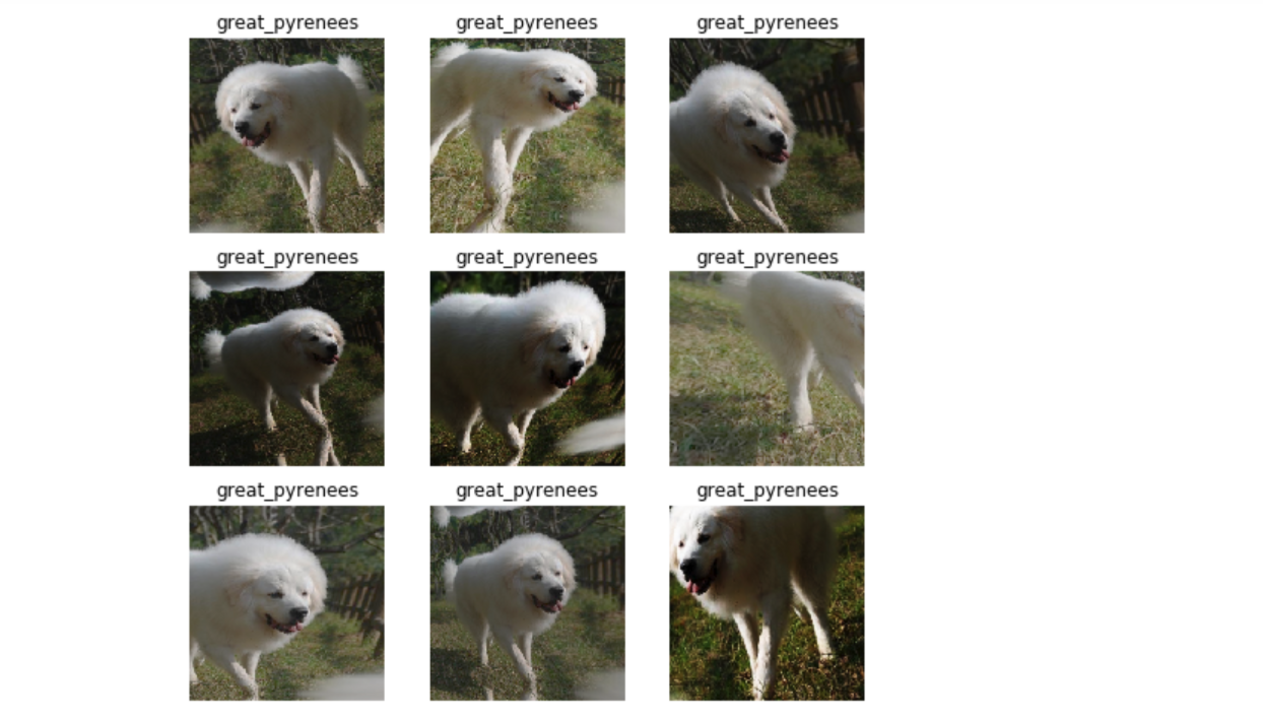
After the first lesson you’ll be able to train a state-of-the-art image classification model on your own data. After completing this lesson, some students from the in-person version of this course (where this material was recorded) published new state-of-the-art results in various domains! The focus for the first half of the course is on practical techniques, showing only the theory required to actually use these techniques in practice. Then, in the second half of the course, we dig deeper and deeper into the theory, until by the final lesson we will build and train a “resnet” neural network from scratch which approaches state-of-the-art accuracy.
The key applications covered are:
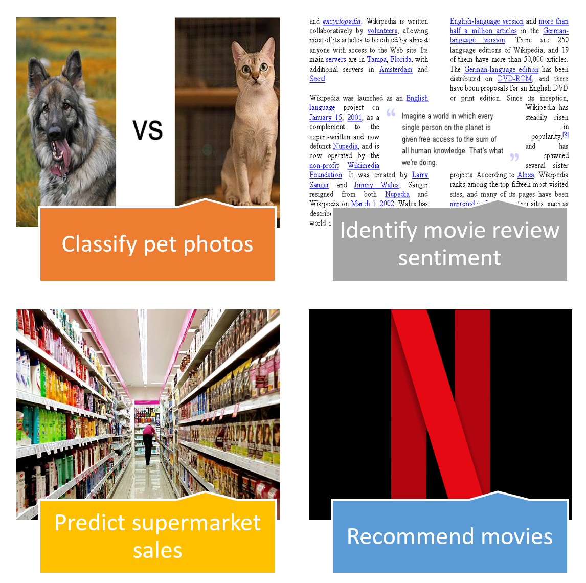
- Computer vision (e.g. classify pet photos by breed)
- Image classification
- Image localization (segmentation and activation maps)
- Image key-points
- NLP (e.g. movie review sentiment analysis)
- Language modeling
- Document classification
- Tabular data (e.g. sales prediction)
- Categorical data
- Continuous data
- Collaborative filtering (e.g. movie recommendation)
We also cover all the necessary foundations for these applications.
We teach using the PyTorch library, which is the most modern and flexible widely-used library available, and we’ll also use the fastai wrapper for PyTorch, which makes it easier to access recommended best practices for training deep learning models (whilst making all the underlying PyTorch functionality directly available too). We think fastai is great, but we’re biased because we made it… but it’s the only general deep learning toolkit featured on pytorch.org, has over 10,000 GitHub stars, and is used in many competition victories, academic papers, and top university courses, so it’s not just us that like it! Note that the concepts you learn will apply equally well to any work you want to do with Tensorflow/keras, CNTK, MXNet, or any other deep learning library; it’s the concepts which matter. Learning a new library just takes a few days if you understand the concepts well.
One particularly useful addition this year is that we now have a super-charged video player, thanks to the great work of Zach Caceres. It allows you to search the lesson transcripts, and jump straight to the section of the video that you find. It also shows links to other lessons, and the lesson summary and resources, in collapsible panes (it doesn’t work well on mobile yet however, so if you want to watch on mobile you can use this Youtube playlist). And an extra big thanks to Sylvain Gugger, who has been instrumental in the development of both the course and the fastai library—we’re very grateful to Amazon Web Services for sponsoring Sylvain’s work.
If you’re interested in giving it a go, click here to go to the course web site. Now let’s look at each lesson in more detail.
Lesson 1: Image classification
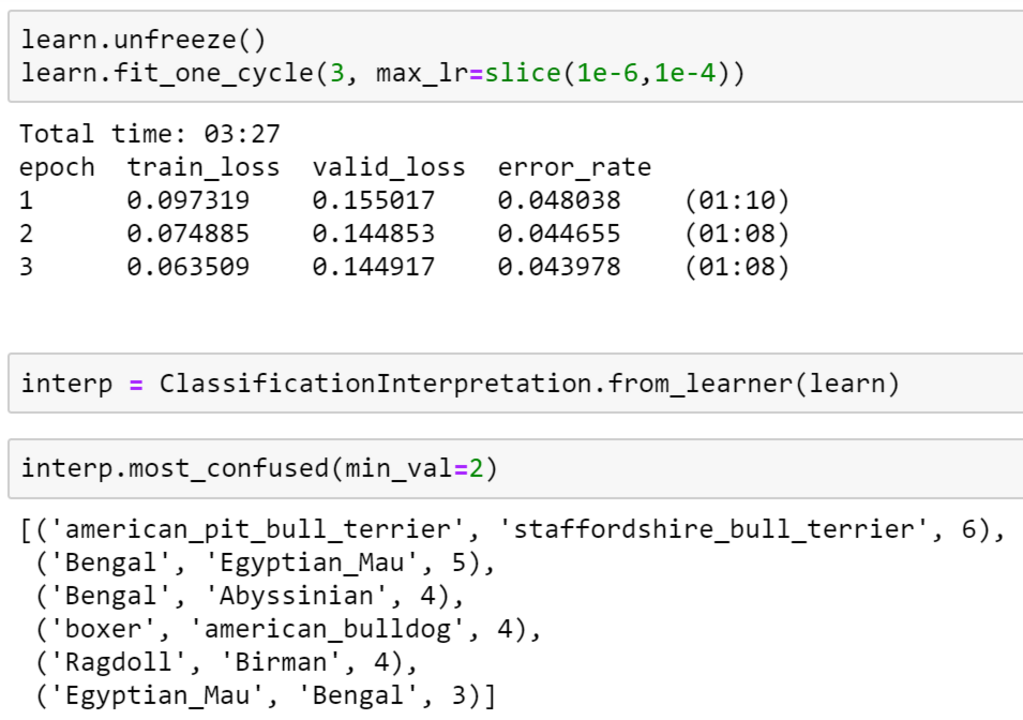
The most important outcome of lesson 1 is that we’ll have trained an image classifier which can recognize pet breeds at state-of-the-art accuracy. The key to this success is the use of transfer learning, which will be a fundamental platform for much of this course. We’ll also see how to analyze the model to understand its failure modes. In this case, we’ll see that the places where the model is making mistakes are in the same areas that even breeding experts can make mistakes.
We’ll discuss the overall approach of the course, which is somewhat unusual in being top-down rather than bottom-up. So rather than starting with theory, and only getting to practical applications later, we start instead with practical applications, and then gradually dig deeper and deeper into them, learning the theory as needed. This approach takes more work for teachers to develop, but it’s been shown to help students a lot, for example in education research at Harvard by David Perkins.
We also discuss how to set the most important hyper-parameter when training neural networks: the learning rate, using Leslie Smith’s fantastic learning rate finder method. Finally, we’ll look at the important but rarely discussed topic of labeling, and learn about some of the features that fastai provides for allowing you to easily add labels to your images.
Note that to follow along with the lessons, you’ll need to connect to a cloud GPU provider which has the fastai library installed (recommended; it should take only 5 minutes or so, and cost under $0.50/hour), or set up a computer with a suitable GPU yourself (which can take days to get working if you’re not familiar with the process, so we don’t recommend it until later). You’ll also need to be familiar with the basics of the Jupyter Notebook environment we use for running deep learning experiments. Up to date tutorials and recommendations for these are available from the course website.
Lesson 2: Data cleaning and production; SGD from scratch
We start today’s lesson by learning how to build your own image classification model using your own data, including topics such as:
- Image collection
- Parallel downloading
- Creating a validation set, and
- Data cleaning, using the model to help us find data problems.
I’ll demonstrate all these steps as I create a model that can take on the vital task of differentiating teddy bears from grizzly bears. Once we’ve got our data set in order, we’ll then learn how to productionize our teddy-finder, and make it available online.
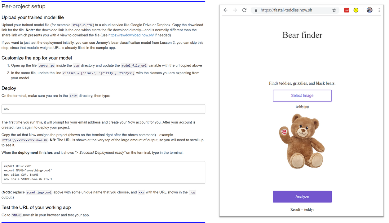
We’ve had some great additions since this lesson was recorded, so be sure to check out:
- The production starter kits on the course web site, such as this one for deploying to Render.com
- The new interactive GUI in the lesson notebook for using the model to find and fix mislabeled or incorrectly-collected images.
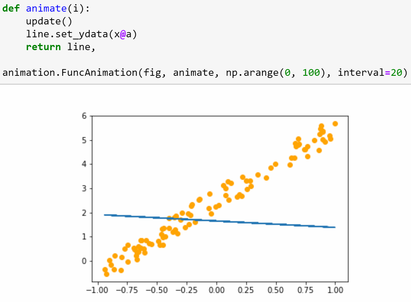
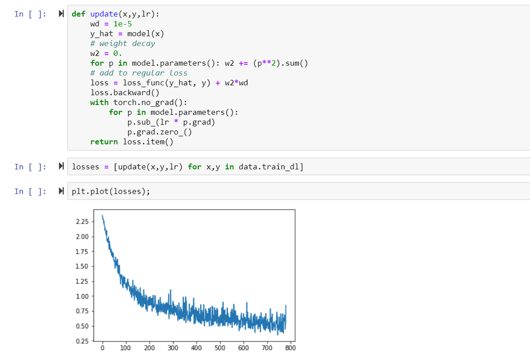
In the second half of the lesson we’ll train a simple model from scratch, creating our own gradient descent loop. In the process, we’ll be learning lots of new jargon, so be sure you’ve got a good place to take notes, since we’ll be referring to this new terminology throughout the course (and there will be lots more introduced in every lesson from here on).
Lesson 3: Data blocks; Multi-label classification; Segmentation
Lots to cover today! We start lesson 3 looking at an interesting dataset: Planet’s Understanding the Amazon from Space. In order to get this data into the shape we need it for modeling, we’ll use one of fastai’s most powerful (and unique!) tools: the data block API. We’ll be coming back to this API many times over the coming lessons, and mastery of it will make you a real fastai superstar! Once you’ve finished this lesson, if you’re ready to learn more about the data block API, have a look at this great article: Finding Data Block Nirvana, by Wayde Gilliam.
One important feature of the Planet dataset is that it is a multi-label dataset. That is: each satellite image can contain multiple labels, whereas previous datasets we’ve looked at have had exactly one label per image. We’ll look at what changes we need to make to work with multi-label datasets.
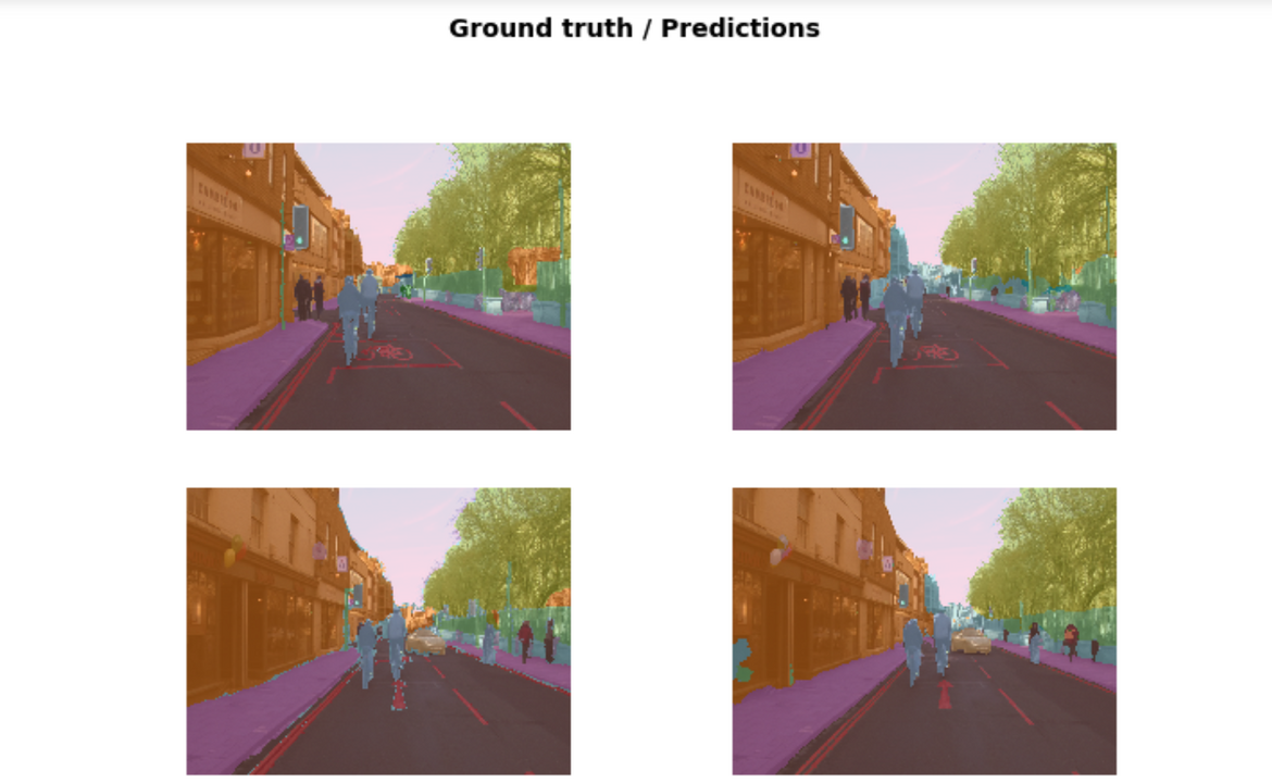
Next, we will look at image segmentation, which is the process of labeling every pixel in an image with a category that shows what kind of object is portrayed by that pixel. We will use similar techniques to the earlier image classification models, with a few tweaks. fastai makes image segmentation modeling and interpretation just as easy as image classification, so there won’t be too many tweaks required.
We will be using the popular CamVid dataset for this part of the lesson. In future lessons, we will come back to it and show a few extra tricks. Our final CamVid model will have dramatically lower error than any model we’ve been able to find in the academic literature!
What if your dependent variable is a continuous value, instead of a category? We answer that question next, looking at a keypoint dataset, and building a model that predicts face keypoints with precision.
Lesson 4: NLP; Tabular data; Collaborative filtering; Embeddings
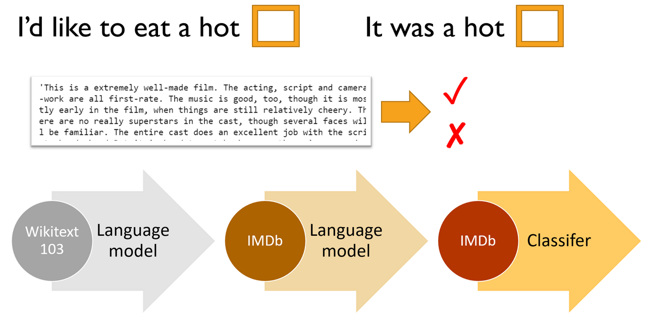
In lesson 4 we’ll dive into natural language processing (NLP), using the IMDb movie review dataset. In this task, our goal is to predict whether a movie review is positive or negative; this is called sentiment analysis. We’ll be using the ULMFiT algorithm, which was originally developed during the fast.ai 2018 course, and became part of a revolution in NLP during 2018 which led the New York Times to declare that new systems are starting to crack the code of natural language. ULMFiT is today the most accurate known sentiment analysis algorithm.
The basic steps are:
- Create (or, preferred, download a pre-trained) language model trained on a large corpus such as Wikipedia (a “language model” is any model that learns to predict the next word of a sentence)
- Fine-tune this language model using your target corpus (in this case, IMDb movie reviews)
- Remove the encoder in this fine tuned language model, and replace it with a classifier. Then fine-tune this model for the final classification task (in this case, sentiment analysis).
After our journey into NLP, we’ll complete our practical applications for Practical Deep Learning for Coders by covering tabular data (such as spreadsheets and database tables), and collaborative filtering (recommendation systems).
For tabular data, we’ll see how to use categorical and continuous variables, and how to work with the fastai.tabular module to set up and train a model.
Then we’ll see how collaborative filtering models can be built using similar ideas to those for tabular data, but with some special tricks to get both higher accuracy and more informative model interpretation.
This brings us to the half-way point of the course, where we have looked at how to build and interpret models in each of these key application areas:
- Computer vision
- NLP
- Tabular
- Collaborative filtering
For the second half of the course, we’ll learn about how these models really work, and how to create them ourselves from scratch. For this lesson, we’ll put together some of the key pieces we’ve touched on so far:
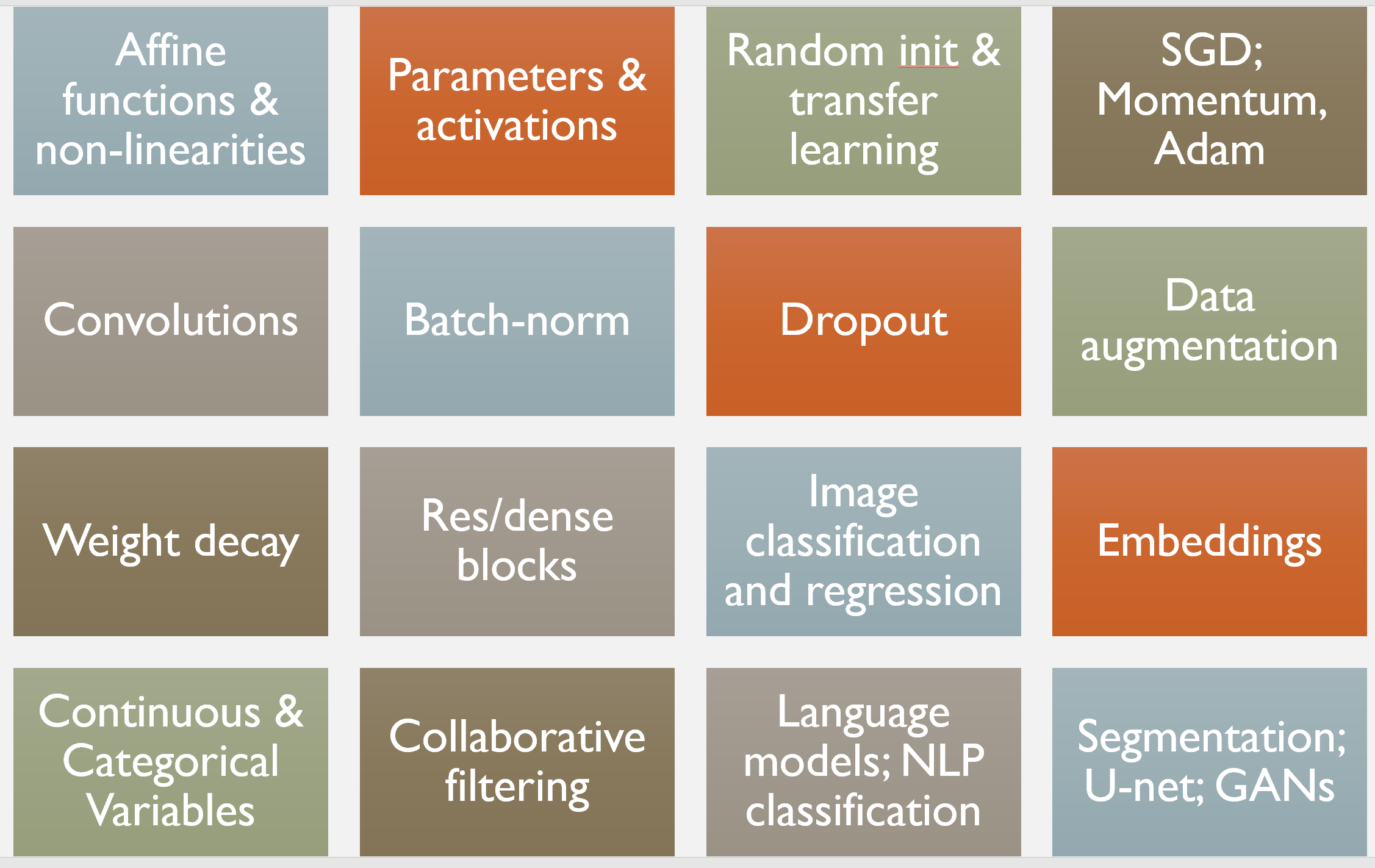
- Activations
- Parameters
- Layers (affine and non-linear)
- Loss function.
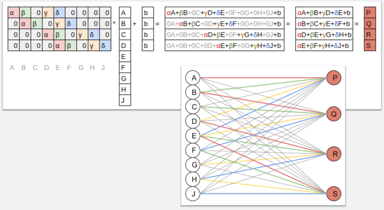
We’ll be coming back to each of these in lots more detail during the remaining lessons. We’ll also learn about a type of layer that is important for NLP, collaborative filtering, and tabular models: the embedding layer. As we’ll discover, an “embedding” is simply a computational shortcut for a particular type of matrix multiplication (a multiplication by a one-hot encoded matrix).
Lesson 5: Back propagation; Accelerated SGD; Neural net from scratch
In lesson 5 we put all the pieces of training together to understand exactly what is going on when we talk about back propagation. We’ll use this knowledge to create and train a simple neural network from scratch.
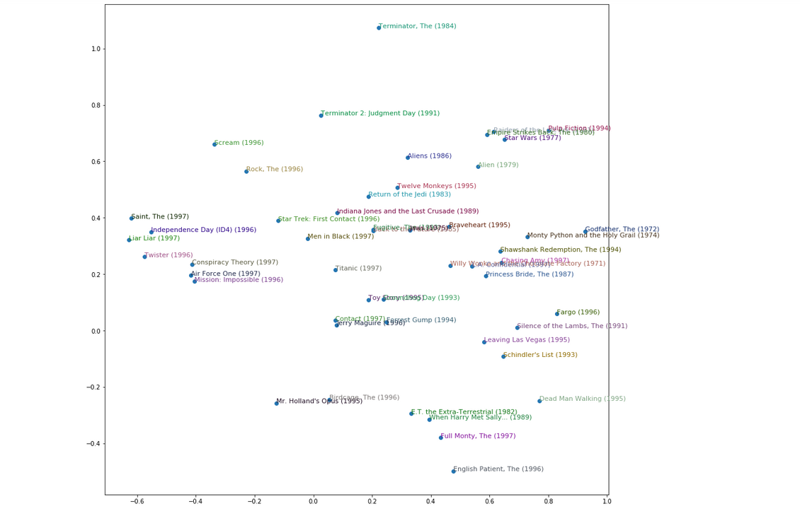
We’ll also see how we can look inside the weights of an embedding layer, to find out what our model has learned about our categorical variables. This will let us get some insights into which movies we should probably avoid at all costs…
Although embeddings are most widely known in the context of word embeddings for NLP, they are at least as important for categorical variables in general, such as for tabular data or collaborative filtering. They can even be used with non-neural models with great success.
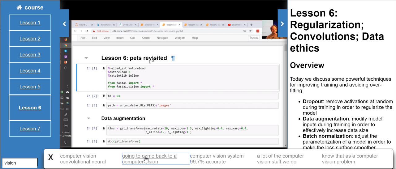
Lesson 6: Regularization; Convolutions; Data ethics
Today we discuss some powerful techniques for improving training and avoiding over-fitting:
- Dropout: remove activations at random during training in order to regularize the model
- Data augmentation: modify model inputs during training in order to effectively increase data size
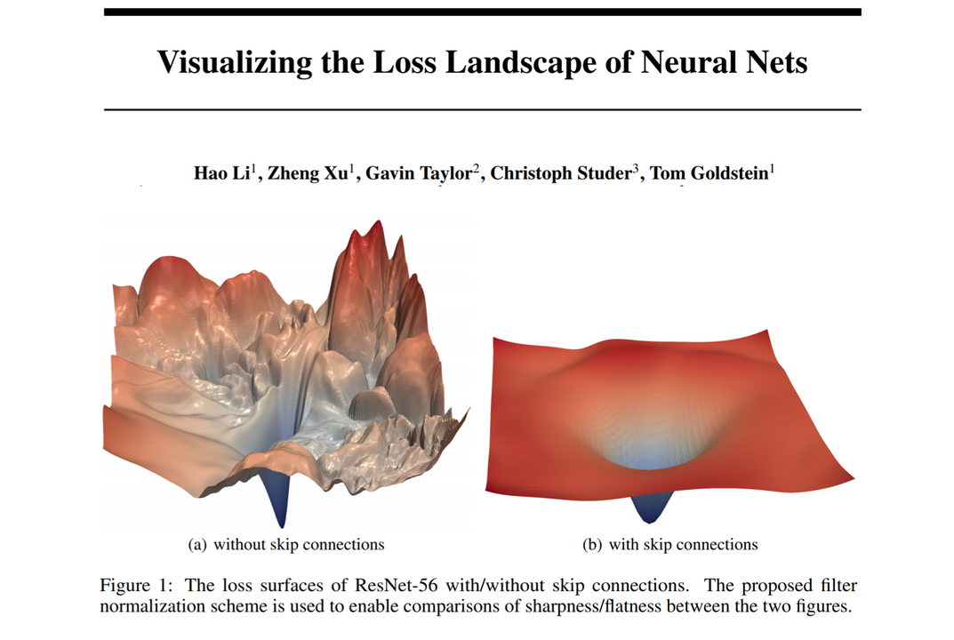
- Batch normalization: adjust the parameterization of a model in order to make the loss surface smoother.
Next up, we’ll learn all about convolutions, which can be thought of as a variant of matrix multiplication with tied weights, and are the operation at the heart of modern computer vision models (and, increasingly, other types of models too).
We’ll use this knowledge to create a class activated map, which is a heat-map that shows which parts of an image were most important in making a prediction.
Finally, we’ll cover a topic that many students have told us is the most interesting and surprising part of the course: data ethics. We’ll learn about some of the ways in which models can go wrong, with a particular focus on feedback loops, why they cause problems, and how to avoid them. We’ll also look at ways in which bias in data can lead to biased algorithms, and discuss questions that data scientists can and should be asking to help ensure that their work doesn’t lead to unexpected negative outcomes.

Lesson 7: Resnets from scratch; U-net; Generative (adversarial) networks
In the final lesson of Practical Deep Learning for Coders we’ll study one of the most important techniques in modern architectures: the skip connection. This is most famously used in the resnet, which is the architecture we’ve used throughout this course for image classification, and appears in many cutting-edge results. We’ll also look at the U-net architecture, which uses a different type of skip connection to greatly improve segmentation results (and also for similar tasks where the output structure is similar to the input).
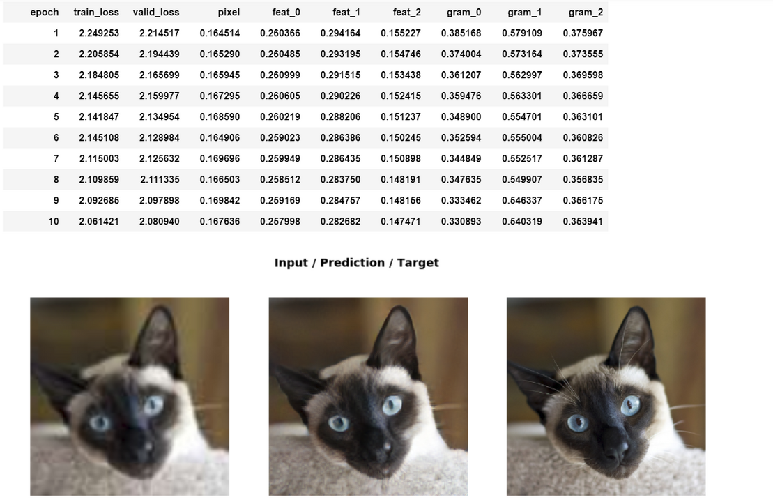
We’ll then use the U-net architecture to train a super-resolution model. This is a model which can increase the resolution of a low-quality image. Our model won’t only increase resolution—it will also remove jpeg artifacts and unwanted text watermarks.
In order to make our model produce high quality results, we will need to create a custom loss function which incorporates feature loss (also known as perceptual loss), along with gram loss. These techniques can be used for many other types of image generation task, such as image colorization.
We’ll learn about a recent loss function known as generative adversarial loss (used in generative adversarial networks, or GANs), which can improve the quality of generative models in some contexts, at the cost of speed.
The techniques we show in this lesson include some unpublished research that:
- Let us train GANs more quickly and reliably than standard approaches, by leveraging transfer learning
- Combines architectural innovations and loss function approaches that haven’t been used in this way before.
The results are stunning, and train in just a couple of hours (compared to previous approaches that take a couple of days).
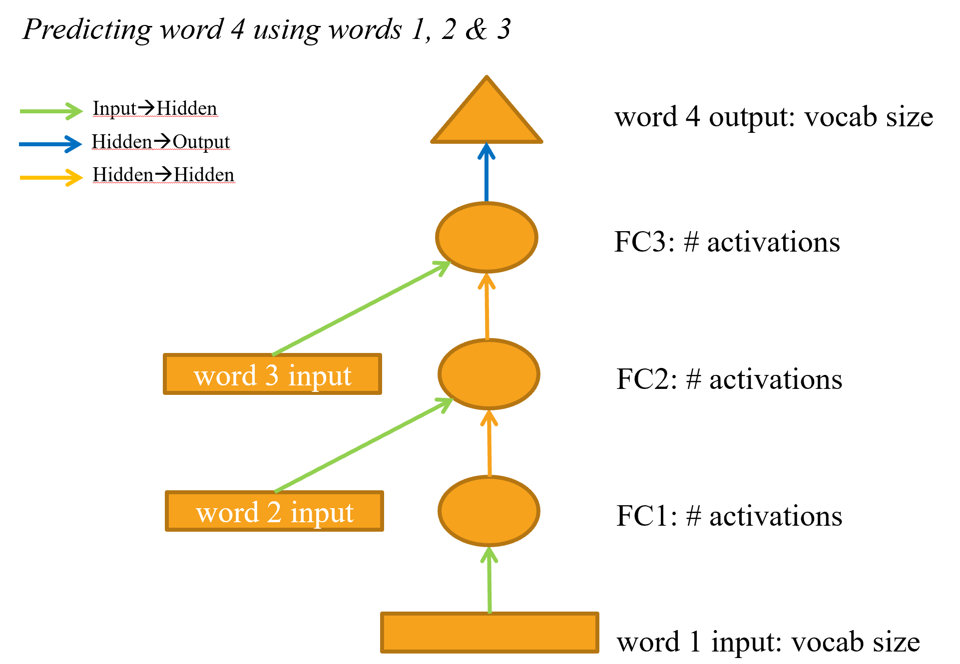
Finally, we’ll learn how to create a recurrent neural net (RNN) from scratch. This is the foundation of the models we have been using for NLP throughout the course, and it turns out they are a simple refactoring of a regular multi-layer network.
Thanks for reading! If you’ve gotten this far, then you should probably head over to course.fast.ai and start watching the first video!