We presented this work at the Facebook f8 conference. You can see this video of our talk here, or read on for more details and examples.
Decrappification, DeOldification, and Super Resolution
In this article we will introduce the idea of “decrappification”, a deep learning method implemented in fastai on PyTorch that can do some pretty amazing things, like… colorize classic black and white movies—even ones from back in the days of silent movies, like this:
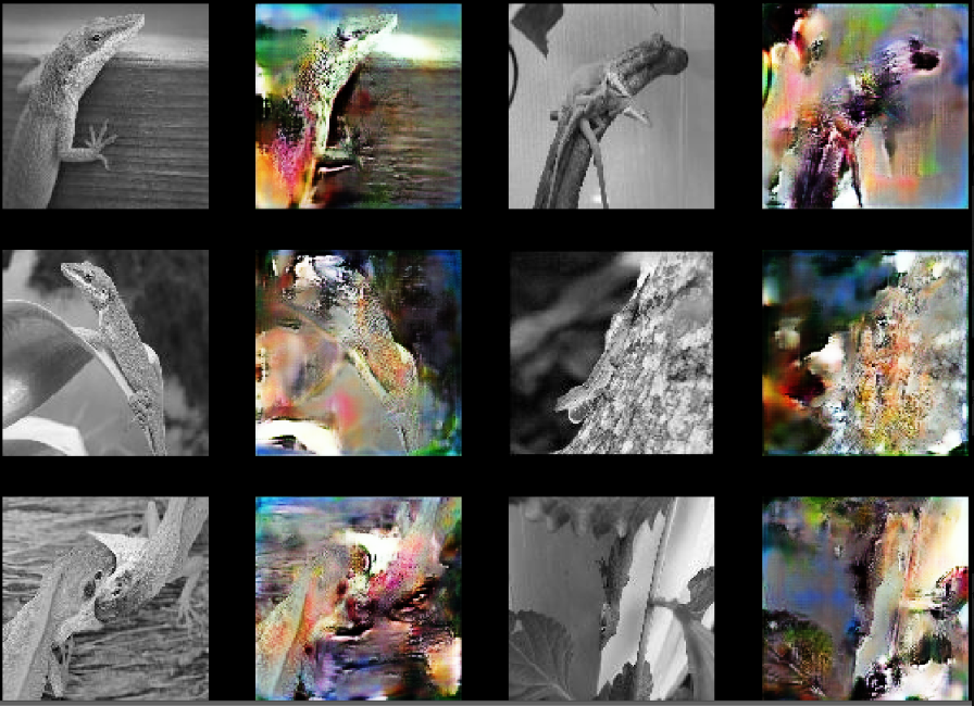
The same approach can make your old family photos look like they were taken on a modern camera, and even improve the clarity of microscopy images taken with state of the art equipment at the Salk Institute, resulting in 300% more accurate cellular analysis.
The genesis of decrappify
Generative models are models that generate music, images, text, and other complex data types. In recent years generative models have advanced at an astonishing rate, largely due to deep learning, and particularly due to generative adversarial models (GANs). However, GANs are notoriously difficult to train, due to requiring a large amount of data, needing many GPUs and a lot of time to train, and being highly sensitive to minor hyperparameter changes.
fast.ai has been working in recent years towards making a range of models easier and faster to train, with a particular focus on using transfer learning. Transfer learning refers to pre-training a model using readily available data and quick and easy to calculate loss functions, and then fine-tuning that model for a task that may have fewer labels, or be more expensive to compute. This seemed like a potential solution to the GAN training problem, so in late 2018 fast.ai worked on a transfer learning technique for generative modeling.
The pre-trained model that fast.ai selected was this: Start with an image dataset and “crappify” the images, such as reducing the resolution, adding jpeg artifacts, and obscuring parts with random text. Then train a model to “decrappify” those images to return them to their original state. fast.ai started with a model that was pre-trained for ImageNet classification, and added a U-Net upsampling network, adding various modern tweaks to the regular U-Net. A simple fast loss function was initially used: mean squared pixel error. This U-Net could be trained in just a few minutes. Then, the loss function was replaced was a combination of other loss functions used in the generative modeling literature (more details in the f8 video) and trained for another couple of hours. The plan was then to finally add a GAN for the last few epochs - however it turned out that the results were so good that fast.ai ended up not using a GAN for the final models.
The genesis of DeOldify
DeOldify was developed at around the same time that fast.ai started looking at decrappification, and was designed to colorize black and white photos. Jason Antic watched the Spring 2018 fast.ai course that introduced GANs, U-Nets, and other techniques, and wondered about what would happen if they were combined for the purpose of colorization. Jason’s initial experiments with GANs were largely a failure, so he tried something else - the self-attention GAN (SAGAN). His ambition was to be able to successfully colorize real world old images with the noise, contrast, and brightness problems caused by film degradation. The model needed to be trained on photos with these problems simulated. To do this, he started with the images in the ImageNet dataset, converted them to b&w, and then added random contrast, brightness, and other changes. In other words, he was “crappifying” images too!
The results were amazing, and people all over the internet were talking about Jason’s new “DeOldify” program. Jeremy saw some of the early results and was excited to see that someone else was getting great results in image generation. He reached out to Jason to learn more. Jeremy and Jason soon realized that they were both using very similar techniques, but had both developed in some different directions too. So they decided to join forces and develop a decrappification process that included all of their best ideas.
The result of joining forces was a process that allowed GANs to be skipped entirely, and which can be trained on a gaming pc. All of Jason’s development was done on a Linux box in a dining room, and each experiment used only a single consumer GPU (a GeForce 1080Ti). The lack of impressive hardware and industrial resources didn’t prevent highly tangible progress. In fact, it probably encouraged it.
Jason then took the process even further, moving from still images to movies. He discovered that just a tiny bit of GAN fine-tuning on top of the process developed with fast.ai could create colorized movies in just a couple of hours, at a quality beyond any automated process that had been built before.
The genesis of microscopy super-resolution
Meanwhile, Uri Manor, Director of the Waitt Advanced Biophotonics Core (WABC) at the Salk Institute, was looking for ways to simultaneously improve the resolution, speed, and signal-to-noise of the images taken by the WABC’s state of the art ZEISS scanning electron and laser scanning confocal microscopes. These three parameters are notably in tension with one another - a variant of the so-called “triangle of compromise”, the bane of existence for all photographers and imaging scientists alike. The advanced microscopes at the WABC are heavily used by researchers at the Salk (as well as several neighboring institutions including Scripps and UCSD) to investigate the ultrastructural organization and dynamics of life, ranging anywhere from carbon capturing machines in plant tissues to synaptic connections in brain circuits to energy generating mitochondria in cancer cells and neurons. The scanning electron microscope is distinguished by its ability to serially slice and image an entire block of tissue, resulting in a 3-dimensional volumetric dataset at nearly nanometer resolution. The so-called “Airyscan” scanning confocal microscopes at the WABC boast a cutting-edge array of 32 hexagonally packed detectors that facilitate fluorescence imaging at nearly double the resolution of a normal microscope while also providing 8-fold sensitivity and speed.
Thanks to the Wicklow AI Medical Research Initiative (WAMRI), Jeremy Howard and Fred Monroe were able to visit Salk to see some of the amazing work done there, and discuss opportunities to use deep learning to help with some of Salk’s projects. Upon meeting Uri, it was immediately clear that fast.ai’s techniques would be a great fit for Uri’s needs for higher resolution microscopy. Fred, Uri, and a Salk-led team of scientists ranging from UCSD to UT-Austin, worked together to bring the methods into the microscopy domain, and the results were stunning. Using carefully acquired high resolution images for training, the group validated “generalized” models for super-resolution processing of electron and fluorescence microscope images, enabling faster imaging with higher throughput, lower sample damage, and smaller file sizes than ever reported. Since the models are able to restore images acquired on relatively low-cost microscopes, this model also presents an opportunity to “democratize” high resolution imaging to those not working at elite institutions that can afford the latest cutting edge instrumentation.
For creating microscopy movies, Fred used a different approach to the one Jason used for classic Hollywood movies. Taking inspiration from this blog post about stabilizing neural style transfer in video, he was able to add a “stability” measure to the loss function being used for creating single image super-resolution. This stability loss measure encourages images with stable features in the face of small amounts of random noise. Noise injection is already part of the process to create training sets at Salk anyways - so this was an easy modification. This stability when combined with information about the preceding and following frames of video significantly reduces flicker and improves the quality of output when processing low resolution movies. See more details about the process in the section below - “Notes on Creating Super-resolution Microscopy Videos”.
A deep dive into DeOldify
Let’s look at what’s going on behind the scenes of DeOldify in some detail. But first, here’s how you can use DeOldify yourself! The easiest way is to use these free Colab notebooks, that run you thru the whole process:
Image Colorization Notebook | Video Colorization Notebook
Or you can download the code and run it locally from the GitHub repo.
Advances in the state of the art
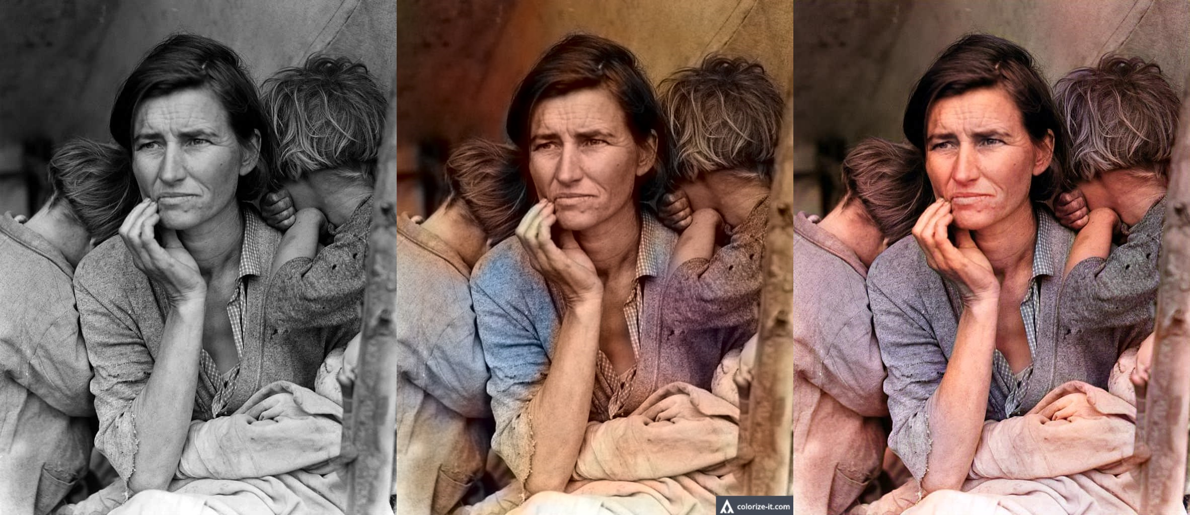
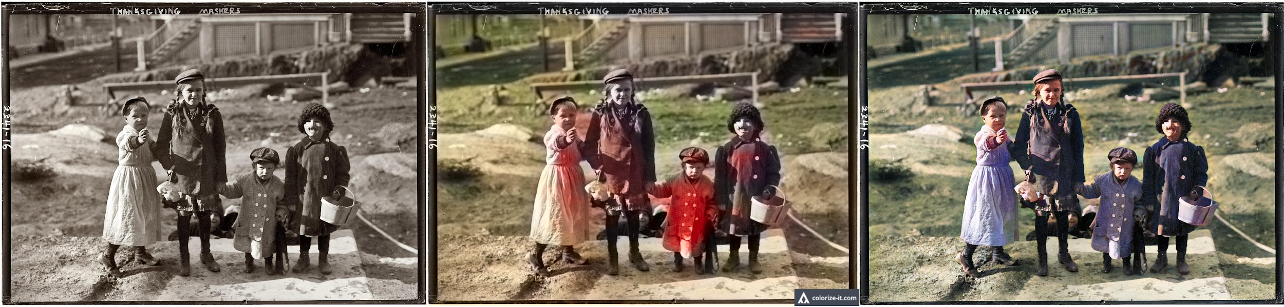
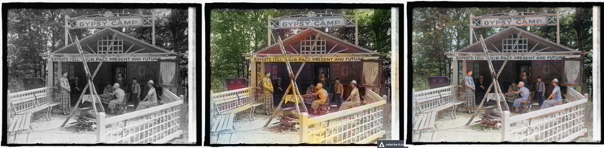
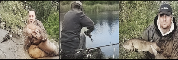
The Zhang et al “Colorful Image Colorization” model is currently popular, widely used, and was previously state of the art. What follows are original black and white photos (left), along with comparisons between the “Colorful Image Colorization” model (middle), and the latest version of DeOldify (right). Notice that the people and objects in the DeOldify photos are colorized more consistently, accurately, and in greater detail. Often, the images that DeOldify produces can be considered nearly photorealistic.
Additionally, high quality video colorization in DeOldify is made possible by advances in training that greatly increase stability and quality of rendering, largely brought about by employing NoGAN training. The following clips illustrate just how well DeOldify not only colorizes video (even special effects!), but also maintains temporal consistency across frames.
The Design of DeOldify
There are a few key design decisions in DeOldify that make a significant impact on the quality of rendered images.
Self-Attention
One of the most important design choices of DeOldify is the use of self-attention, as implemented in the “Self-Attention Generative Adversarial Networks” (SAGAN) paper. The paper summarizes the motivation for using them:
“Traditional convolutional GANs generate high-resolution details as a function of only spatially local points in lower-resolution feature maps. In SAGAN, details can be generated using cues from all feature locations. Moreover, the discriminator can check that highly detailed features in distant portions of the image are consistent with each other.”
This same approach was adapted to the critic and U-Net based generators used in DeOldify. The motivation is simple: You want to have maximal continuity, consistency, and completeness in colorization, and self-attention is vital for this. This becomes a particularly apparent problem in models without self-attention when you attempt to colorize images containing large features such as ocean water. Often, you’ll see these large areas filled in with inconsistent coloration in such models.
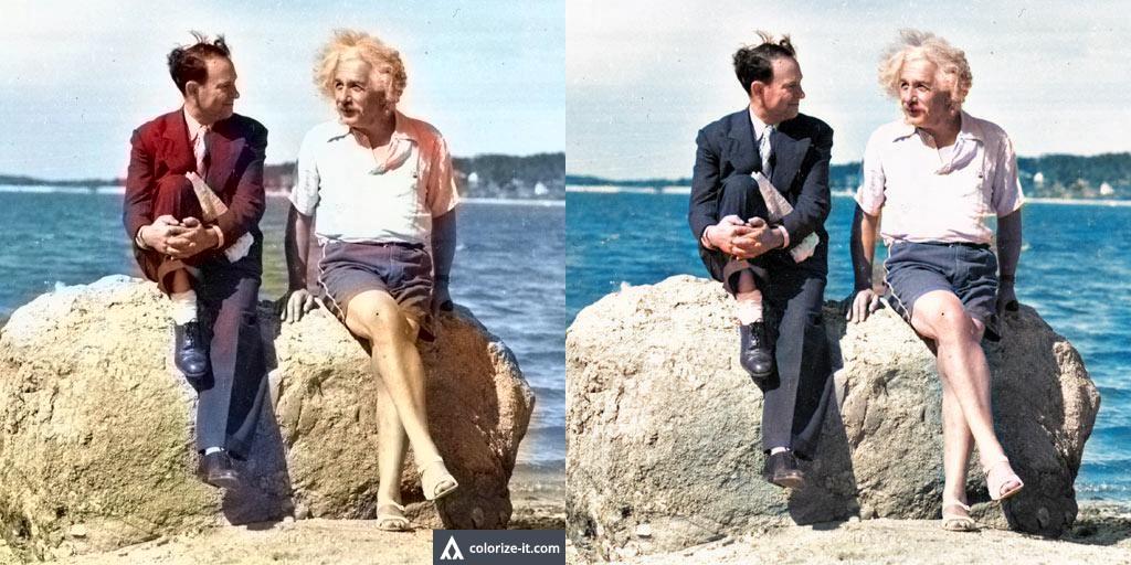
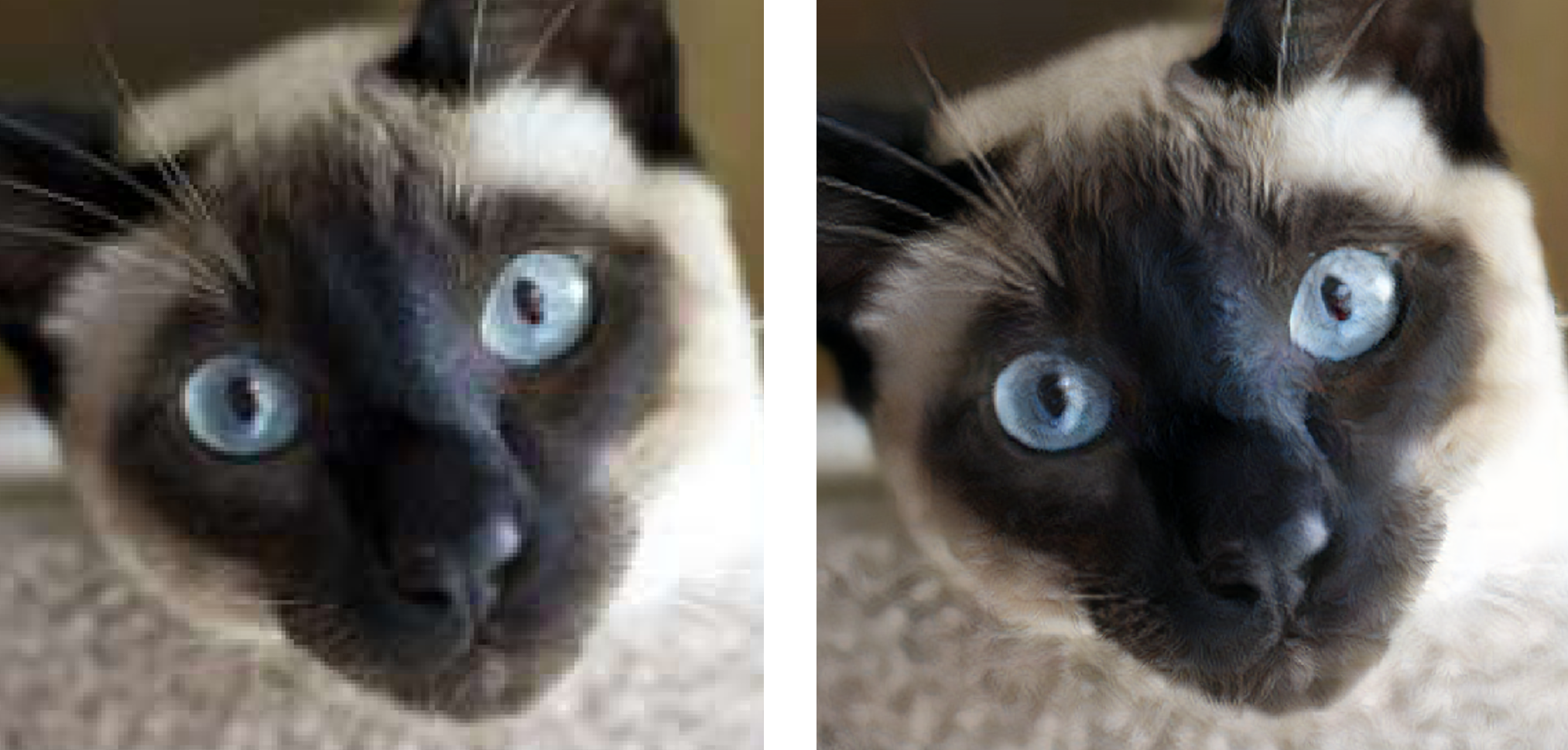
Zhang et al “Colorful Image Colorization” model output is on the left, and DeOldify output is on the right. Notice that the water in the background, as well as the clothing of the man on the left, is much more consistently, completely, and correctly colorized in the DeOldify model. This is thanks in large part to self-attention, by which colorization decisions can easily take into account a more global context of features.
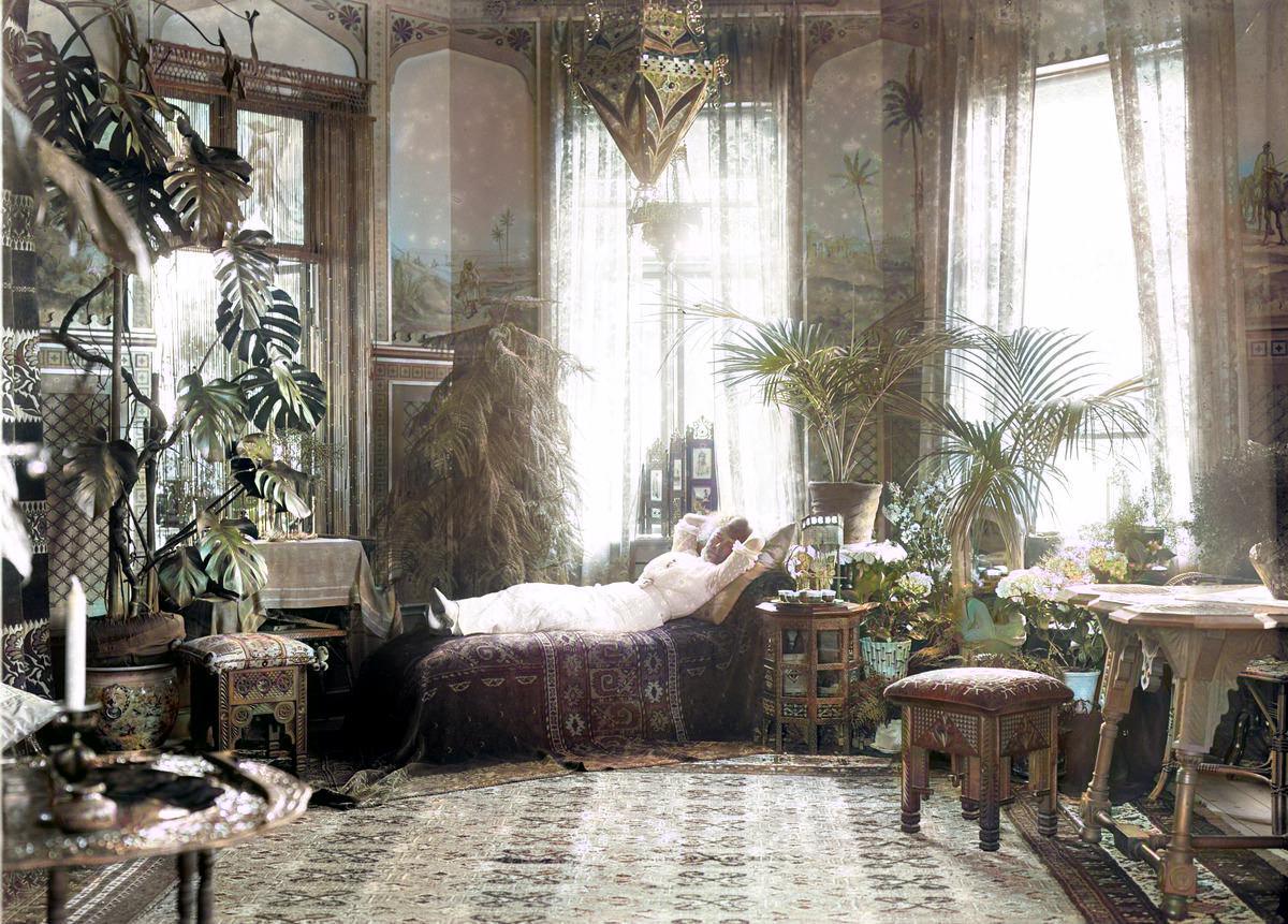
Self-attention also helps drive fantastic levels of detail in the colorizations.
Reliable Feature Detection
In contrast to other colorization models, DeOldify uses custom U-Nets with pretrained resnet backbones for each of its generator models. These are based on Fast.AI’s well-designed DynamicUnet, with a few minor modifications. The deviations from standard U-Nets include the aforementioned self-attention, as well as the addition of spectral normalization. These changes were modeled after the work done in the “Self-Attention Generative Adversarial Networks” paper.
The “video” and “stable” models use a resnet101 backbone and the decoder side emphasizes width (number of filters) over depth (number of layers). This configuration has proven to support the most stable and reliable renderings seen so far. In contrast, the “artistic” model has a resnet34 backbone and the decoder side emphasizes depth over width. This configuration is great for creating interesting colorizations and highly detailed renders, but at the cost of being more inconsistent in rendering than the “stable” and “video” models.
There are two primary underlying motivations for using a pretrained U-Net. First, it saves unnecessary training time that a large task in colorization is already trained for free- object recognition. That’s ImageNet-based object recognition, which for a single GPU will take at least a few days to train from scratch. Instead, we’re just fine-tuning that pretrained network to fit our task, which is much less work. Additionally, the U-Net architecture, especially Fast.AI’s DynamicUnet, is simply superior in image generation applications. This is due to key detail preserving and enhancing features like cross connections from encoder to decoder, learnable blur, and pixel shuffle. The resnet backbone itself is well-suited for the task of scene feature recognition.
To further encourage robustness in dealing with old and low quality images and film, we train with fairly extreme brightness and contrast augmentations. We’ve also employed gaussian noise augmentation in video model training in order to reduce model sensitivity to meaningless noise (grain) in film.
When feature recognition fails, jarring render failures such as “zombie hands” can result.
NoGAN Training
NoGAN is a new and exciting technique in GAN training that we developed, in pursuit of higher quality and more stable renders. How, and how well, it works is a bit surprising.
Here is the NoGAN training process:
Pretrain the Generator. The generator is first trained in a more conventional and easier to control manner - with Perceptual Loss (aka Feature Loss) by itself. GAN training is not introduced yet. At this point you’re training the generator as best as you can in the easiest way possible. This takes up most of the time in NoGAN training. Keep in mind: this pretraining by itself will get the generator model far. Colorization will be well-trained as a task, albeit the colors will tend toward dull tones. Self-Attention will also be well-trained at the at this stage, which is very important.
Save Generated Images From Pretrained Generator.
Pretrain the Critic as a Binary Classifier. Much like in pretraining the generator, what we aim to achieve in this step is to get as much training as possible for the critic in a more “conventional” manner which is easier to control. And there’s nothing easier than a binary classifier! Here we’re training the critic as a binary classifier of real and fake images, with the fake images being those saved in the previous step. A helpful thing to keep in mind here is that you can simply use a pre-trained critic used for another image-to-image task and refine it. This has already been done for super-resolution, where the critic’s pretrained weights were loaded from that of a critic trained for colorization. All that is needed to make use of the pre-trained critic in this case is a little fine-tuning.
Train Generator and Critic in (Almost) Normal GAN Setting. Quickly! This is the surprising part. It turns out that in this pretraining scenario, the critic will rapidly drive adjustments in the generator during GAN training. This happens during a narrow window of time before an “inflection point” of sorts is hit. After this point, there seems to be little to no benefit in training any further in this manner. In fact, if training is continued after this point, you’ll start seeing artifacts and glitches introduced in renderings.
In the case of DeOldify, training to this point requires iterating through only about 1% to 3% of ImageNet data (or roughly 2600 to 7800 iterations on a batch size of five). This amounts to just around 30-90 minutes of GAN training, which is in stark contrast to the three to five days of progressively-sized GAN training that was done previously. Surprisingly, during that short amount of training, the change in the quality of the renderings is dramatic. In fact, this makes up the entirety of GAN training for the video model. The “artistic” and “stable” models go one step further and repeat the the NoGAN training process steps 2-4 until there’s no more apparent benefit (around five repeats).
Note: a small but significant change to this GAN training that deviates from conventional GANs is the use of a loss threshold that must be met by the critic before generator training commences. Until then, the critic continues training to “catch up” in order to be able to provide the generator with constructive gradients. This catch up chiefly takes place at the beginning of GAN training which immediately follows generator and critic pretraining.
Note that the frame at 1.4% is considered to be just before the “inflection point” - after this point, artifacts and incorrect colorization start to be introduced. In this case, the actors’ skin becomes increasingly orange and oversaturated, which is undesirable. These were generated using a learning rate of 1e-5. The current video model of DeOldify was trained at a learning rate of 5e-6 to make it easier to find the “inflection point”.
Research on NoGAN training is still ongoing, so there are still quite a few questions to investigate. First, the technique seems to accommodate small batch sizes well. The video model was trained using a batch size of 5 (and the model uses batch normalization). However, there’s still the issue of artifacts and discoloration being introduced after the “inflection point”, and it’s suspected that this could be reduced or eliminated by mitigating batch size related issues. This could be done either by increasing batch size, or perhaps by using normalization that isn’t affected by batch size. It may very well be that once these issues are addressed, additional productive training can be accomplished before hitting a point of diminishing returns.
Another open question with NoGAN is how broadly applicable the approach is. It stands to reason that this should work well for most image-to-image tasks, and even perhaps non-image related training. However, this simply hasn’t yet been explored enough to draw strong conclusions. We did get interesting and impressive results on applying NoGAN to superresolution. In just fifteen minutes of direct GAN training (or 1500 iterations), the output of Fast.AI’s Part 1 Lesson 7 Feature Loss based super resolution training is noticeably sharpened (original lesson Jupyter notebook here).
Finally, the best practices for NoGAN training haven’t yet been fully explored. It’s worth mentioning again that the “artistic” and “stable” models were trained on not just one, but repeated cycles of NoGAN. What’s still unknown is just how many repeats are possible to still get a benefit, and how to make the training process less tedious by automatically detecting an early stopping point just before the “inflection point”. Right now, the determination of the inflection point is a manual process, and consists of a person visually assessing the generated images at model checkpoints. These checkpoints need to be saved at an interval of least every 0.1% of total data—otherwise, it is easily missed. This is definitely tedious, and prone to error.
How Stable Video is Achieved
The Problem – A Flickering Mess
Just a few months ago, the technology to create well-colorized video seemed to be out of reach. If you took the original DeOldify model and merely colorized each frame just as you would any other image, the result was this—a flickering mess:
The immediate solution that usually springs to mind is temporal modeling of some sort, whereby you enforce constraints on the model during training over a window of frames to keep colorization decisions more consistent. This would seem to make sense, but it does add a significant amount of complication, and the not-so-rare cases of changing scenes raises further questions about how to handle continuity. The rabbit hole deepens, and quickly. With these assumptions of needing temporal coherence enforced, the prospect of making seamless and flicker-free colorized video seemed quite far off. Luckily, it turns out these assumptions were wrong.
The Problems Melt Away with NoGAN
A surprising observation that we’ve made while developing DeOldify is that the colorization decisions are not at all arbitrary, even after GAN training and across different models. Rather, different models and training regimes keep arriving at almost the same solution, with only very minor variations in colorization. This even happens with the colorization of things you might expect to be unknowable and unconstrained by the luminance information in black and white photos: Clothing, cars, special effects in movies, etc. We’re not sure yet what exactly the model is learning to be able to more or less deterministically colorize images. But the bottom line is that temporal coherence concerns simply go away when you realize that there’s nothing to track—objects in frames will keep rendering the same regardless.
Additionally, it turns out that in NoGAN training the learning that takes place before the “inflection point” trains the generator in a very effective way. This is not only in terms of quickly achieving good colorization, but also without introducing artifacts, discoloration and inconsistency in generator renders. In other words, those artifacts and glitches in that “flickering mess” render of Metropolis above are coming from too much GAN training, and we can mitigate that pretty much completely with NoGAN!
NoGAN is the most significant element in achieving video render stability, but there’s a few additional design choices that also make an impact. For example, a larger resnet backbone (resnet101) makes a noticeable difference in how accurately and robustly features are detected, and therefore how consistently the frames are rendered as objects and scenes move. Another consideration is render resolution—increasing this makes a positive difference in some cases, but not nearly as big as one may expect. Most of the videos we’ve rendered have been done at resolutions ranging from 224px to 360px, and this tends to work just fine.
The end result of all this is that flicker-free, temporally consistent, and colorful video is achieved simply by rendering individual frame as if they were any other image! There is zero temporal modeling involved.
The DeOldify Graveyard: Things That Didn’t Work
For every design experiment that actually worked, there were at least ten that didn’t. This list is not exhaustive by any stretch but it includes what we consider to be particularly helpful to know.
Wasserstein GAN (WGAN) and Its Variants
The original approach attempted in the development of DeOldify was to base the architecture on Wasserstein GAN (WGAN). It turns out the stability of the WGAN and its subsequent improvements were not sufficient for practical application in colorization. Training would work somewhat for a while, but would invariably diverge from a stable solution as GANs are known to do. To an extent, the results were entertaining. What actually did wind up working extremely well (the first time even) was modeling DeOldify after Self-Attention Generative Adversarial Networks instead.
Various Other Normalization Schemes
The following normalization variations were attempted. None of them worked nearly as well as having batch normalization and spectral normalization combined in the generator, and just spectral normalization in the critic.
- Spectral Normalization Only in Generator. This trained more slowly and was generally more unstable.
- Batchnorm at Output of Generator. This slowed down training significantly and didn’t seem to provide any real benefit.
- Weight Normalization in Generator. Ditto on the slowed training, and images didn’t turn out looking as good either. Interestingly however, it seems like weight normalization works the best when doing NoGAN training for super resolution.
Other Loss Functions
The interaction between the conventional (non-GAN) loss function and the GAN loss/training turns out to be crucial, yet tricky. For one, you have to weigh the non-GAN and GAN losses carefully, and it seems this can only come out of experimentation. The nice thing about NoGAN is that the iterations on this process are very quick relative to other GAN training regimes—it’s a matter of minutes instead of days to see the end result.
Another tricky aspect of the loss interaction is that you can’t just select any non-GAN loss function to work side by side with GAN loss. It turns out that Perceptual Loss (aka Feature Loss) empirically works best for this, especially in comparison to L1 and Mean Squared Error (MSE) loss.
It seems that since most of the emphasis in NoGAN training is in pretraining, it would be especially important to make sure that pretraining is taken as far as possible in rendering quality before making the switch to GAN. Perceptual Loss does just that—by itself, it produces the most colorful results of all the non-GAN losses attempted. In contrast, simpler loss functions such as MSE and L1 loss tend to produce dull colorizations as they encourage the networks to “play it safe” and bet on gray and brown by default.
Additions to perceptual loss were also attempted. Most notable were gram style loss and wasserstein distance. While the two cannot be ruled out and will be revisited in the future, the losses wound up encouraging strange orange and yellow discolorations when present in conjunction with GAN training. It’s suspected that the losses were simply not used effectively.
Reduced Number of Model Parameters
Something that tends to surprise people about DeOldify is the large model size. In the latest iteration, the “video” and “stable” models are set to a width of 1000 filters on the decoder side for most of the layers. The “artistic” model has the number of filters multiplied by 1.5 over the standard DynamicUnet configuration. Similarly, the critic is also rather hefty, with a starting width of 256 as opposed to the more conventional 64 or 128. Many experiments were done attempting to reduce the number of parameters, but they all generally ran into the same problem: The resulting renders were significantly less colorful.
Creating Super-resolution Microscopy Videos
Finally, we’ll discuss some of the details of the approach used at the Salk Institute for creating high resolution microsopy videos. The high level overview of the steps involved in creating model to produce high resolution microscopy videos from low resolution sequences is:
- Acquire high resolution source material for training and low resolution material to be improved.
- Develop a crappifier function
- Create low res training dataset of image-tuples (groups of 3 images)
- Create two training sets, A and B, by applying the crappifier to each image-tuple twice
- Train the model on both training sets simultaneously with “stability” loss
- Use the trained model to generate high resolution videos by running it across real low resolution source material
Acquisition of Source Material
At Salk we have been fortunate because we have produced decent results using only synthetic low resolution data. This is important because it is time consuming and rare to have perfectly aligned pairs of high resolution and low resolution images - and that would be even harder or impossible with video (live cells). In this case the files were acquired in proprietary czi format. Fortunately there is a python based tool for reading this format here.
Developing a Crappifier
In order to produce synthetic training data we need a “crappifier” function. This is a function that transforms a high resolution image into a low resolution image that approximates the real low resolution images we will be working with once our model is trained. The crappifier injects some randomness in the forms of both gaussian and poisson noise. These are both present in microscopy images. We were influenced in this design by the excellent work done by the CSBDeep team.
The crappifier can be simple but does materially impact both the quality and characteristics of output. For example, we found that if our crappifier injected too much high frequency noise into the training data, the trained model would have a tendency to eliminate thin and fine structures like those of neurons.
Generating the Synthetic Low Resolution Data for Training
The next step is to bundle sequences of images and their target together for training like this:
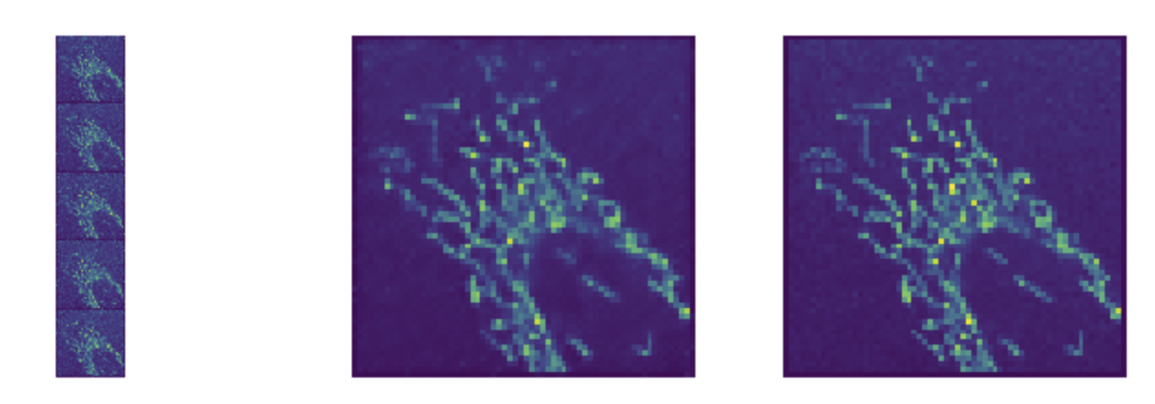
This image shows an example from a training where we are using 5 sequential images ( t-2, t-1, t 0, t+1, t+2) - to predict a single super-resolution output image (also at time t 0 )
For the movies we used bundles of 3 images and predicted the high resolution image at the corresponding middle time. In other words, we predicted super-resolution at time t0 with low resolution images from times t-1, t 0 and t+1.
We chose 3 images because that conveniently allowed us to easily use pre-existing super-resolution network architectures, data loaders and loss functions that were written for 3 channels of input.
Creating a Second Set of Low Resolution Data
To use stability loss we actually have to apply the crappifier function to the source material twice in order to create two parallel datasets. Because the crappifier injects random noise - the two datasets will differ from each other slightly - but have the same high resolution targets. A perfectly stable model would predict identical high resolution output images from both training datasets - while ignoring the random noise.
Training the model with Stability Loss
In addition to the normal loss functions we would use for super-resolution, we need to choose a measure of stability loss. This is a measure of similarity of output generation when appy the model to each of the two training sets which as we explained previously differ only in their application of randomly applied noise.
Given the low resolution image sequence X that we will use to predict the true high resolution image T, we create X1 and X2 which result from to separate applications of the random noise generating crappifier function.
X1 = crappifier(X) and X2 = crappifier(X)
Given our trained model M, we then predict Y1 and Y2 as follows:
Y1 = M(X1) and Y2 = M(X2)
Giving us super resolutions L1 = loss(Y1, T) and L2 = loss(Y2,T). Our stability loss is the difference between the predicted images. We used L1 loss but you could also use a feature loss or some other approach to measure the difference:
LossStable = loss(Y1,Y2)
Our final training loss is therefore: loss = L1 + L2 + LossStable
Generating Movies
Now that we have a trained model, generating high resolution output from low resolution input is simply a matter of running the model across a sliding window of, in this case, three low resolution input images at a time. Imageioin one convenient way to write out multiimage tif files or mp4 files.
Examples:
Real low resolution input | Single frame of input and conventional loss | Multiple frames of input and stability loss penalty