Summary: recently while fine-tuning a large language model (LLM) on multiple-choice science exam questions, we observed some highly unusual training loss curves. In particular, it appeared the model was able to rapidly memorize examples from the dataset after seeing them just once. This astonishing feat contradicts most prior wisdom about neural network sample efficiency. Intrigued by this result, we conducted a series of experiments to validate and better understand this phenomenon. It’s early days, but the experiments support the hypothesis that the models are able to rapidly remember inputs. This might mean we have to re-think how we train and use LLMs.
How neural networks learn
We train neural network classifiers by showing them examples of inputs and outputs, and they learn to predict outputs based on inputs. For example, we show examples of pictures of dogs and cats, along with the breed of each, and they learn to guess the breed from the image. To be more precise, for a list of possible breeds, they output their guess as to the probability of each breed. If it’s unsure, it will guess a roughly equal probability of each possible breed, and if it’s highly confident, it will guess a nearly 1.0 probability of its predicted breed.
The training process consists of every image in a training set being shown to the network, along with the correct label. A pass through all the input data is called an “epoch”. We have to provide many examples of the training data for the model to learn effectively.
During training the neural network attempts to reduce the loss, which is (roughly speaking) a measure of how often the model is wrong, with highly confident wrong predictions penalised the most, and vise versa. We calculate the loss after each batch for the training set, and from time to time (often at the end of each epoch) we also calculated the loss for a bunch of inputs the model does not get to learn from – this is the “validation set”. Here’s what that looks like in practice when we train for 11 epochs:
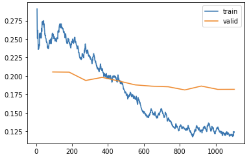
As you see, the training loss gradually (and bumpily) improves relatively quickly, slowing down over time, and the validation loss improves more slowly (and would eventually flatten out entirely, and then eventually get worse, if trained for longer).
You can’t see from the chart where epochs start and stop, because it takes many epochs before a model learns what any particular image looks like. This has been a fundamental constraint of neural networks throughout the decades they’ve been developed – they take an awfully long time to learn anything! It’s actually an area of active research about why neural nets are so “sample inefficient”, especially compared to how children learn.
A very odd loss curve
We have recently been working on the Kaggle LLM Science Exam competition, which “challenges participants to answer difficult science-based questions written by a Large Language Model”. For instance, here’s the first question:
Which of the following statements accurately describes the impact of Modified Newtonian Dynamics (MOND) on the observed “missing baryonic mass” discrepancy in galaxy clusters?
- MOND is a theory that reduces the observed missing baryonic mass in galaxy clusters by postulating the existence of a new form of matter called “fuzzy dark matter.”
- MOND is a theory that increases the discrepancy between the observed missing baryonic mass in galaxy clusters and the measured velocity dispersions from a factor of around 10 to a factor of about 20.
- MOND is a theory that explains the missing baryonic mass in galaxy clusters that was previously considered dark matter by demonstrating that the mass is in the form of neutrinos and axions.
- MOND is a theory that reduces the discrepancy between the observed missing baryonic mass in galaxy clusters and the measured velocity dispersions from a factor of around 10 to a factor of about 2.
- MOND is a theory that eliminates the observed missing baryonic mass in galaxy clusters by imposing a new mathematical formulation of gravity that does not require the existence of dark matter.
For those playing along at home, the correct answer, apparently, is D.
Thankfully, we don’t have to rely on our knowledge of Modified Newtonian Dynamics to answer these questions – instead, we are tasked to train a model to answer these questions. When we submit our model to Kaggle, it will be tested against thousands of “held out” questions that we don’t get to see.
We trained our model for 3 epochs on a big dataset of questions created by our friend Radek Osmulski, and saw the following most unexpected training loss curve:
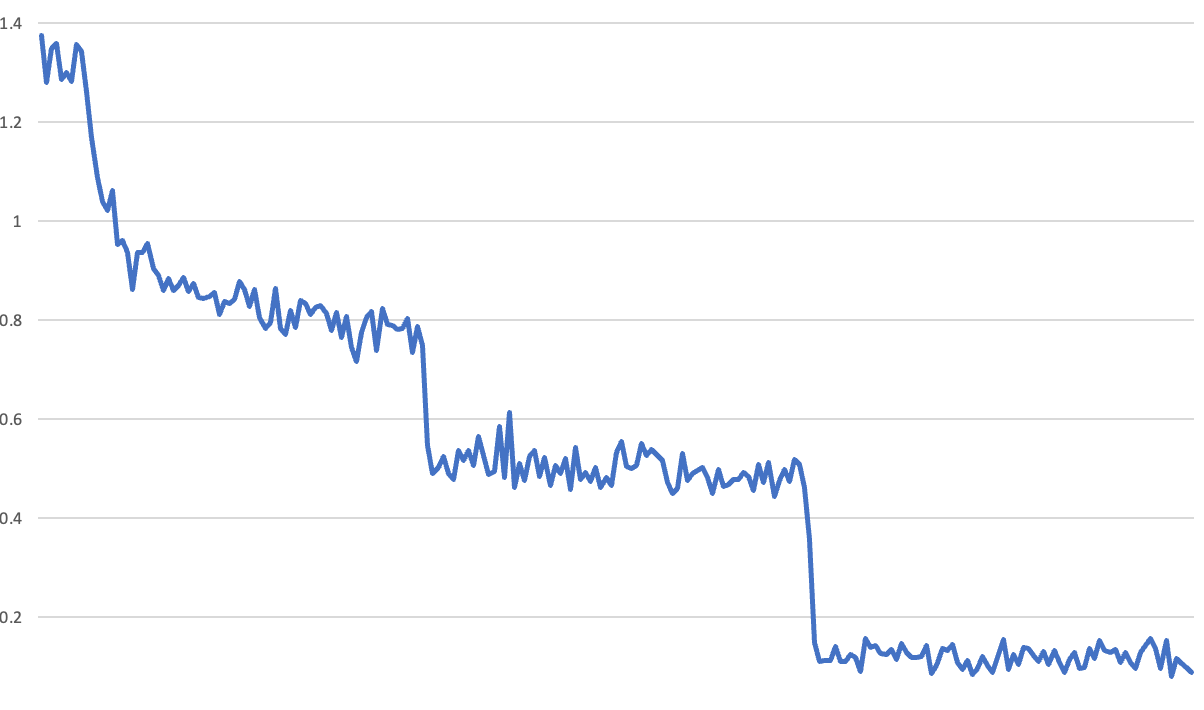
The problem here is that you can clearly see the end of each epoch - there’s a sudden downwards jump in loss. We’ve seen similar loss curves before, and they’ve always been due to a bug. For instance, it’s easy to accidentally have the model continue to learn when evaluating the validation set – such that after validation the model suddenly appears much better. So we set out to look for the bug in our training process. We were using Hugging Face’s Trainer, so we guessed there must be a bug in that.
Whilst we began stepping through the code, we also asked fellow open source developers on the Alignment Lab AI Discord if they’ve seen similar odd training curves, and pretty much everyone said “yes”. But everyone who responded was using Trainer as well, which seemed to support our theory of a bug in that library.
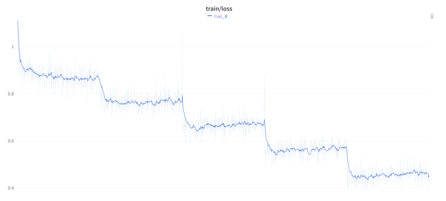
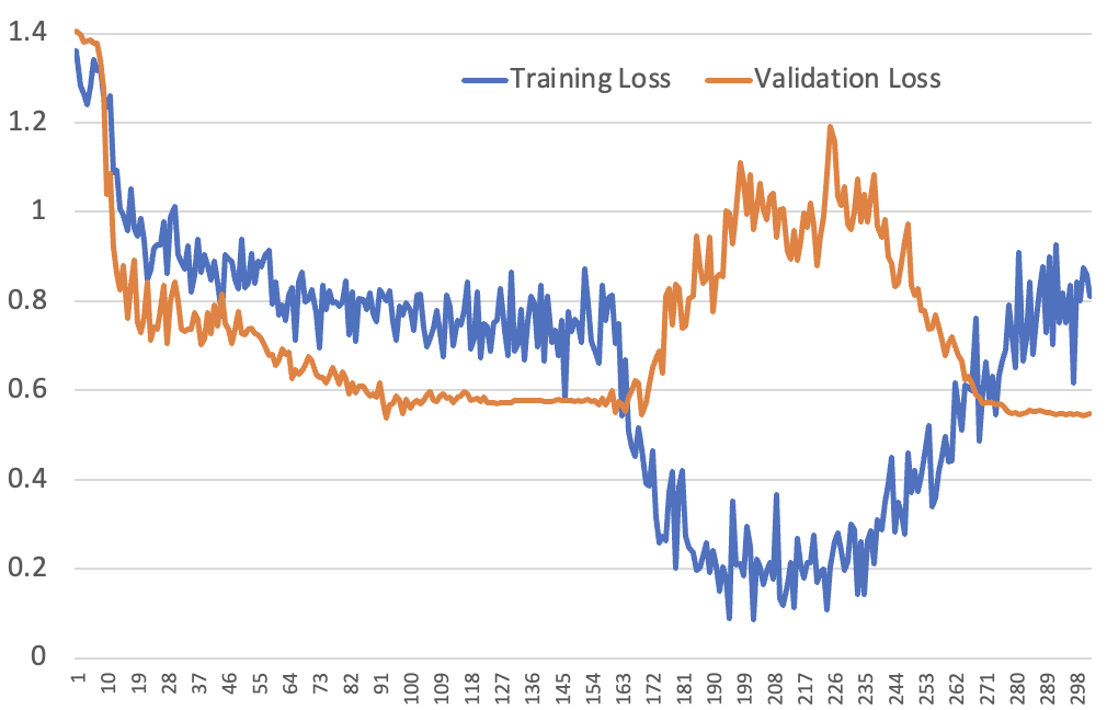
But then @anton on Discord told us he was seeing this curve with his own simple custom training loop:
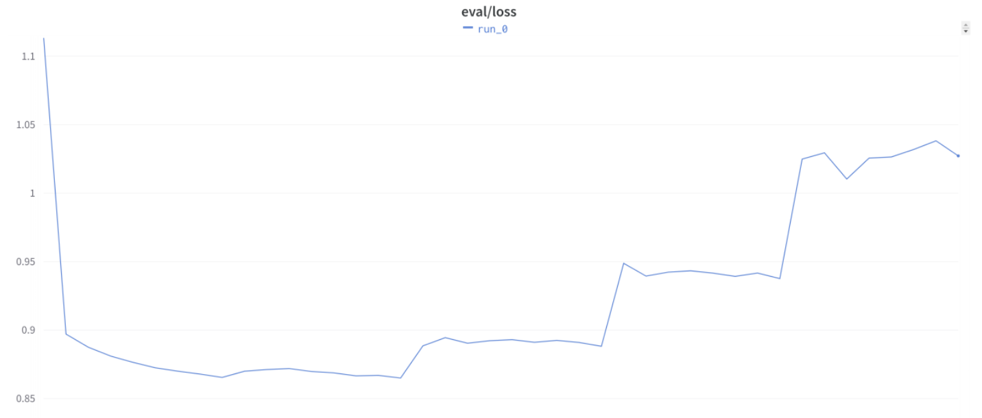
…and he also showed us this accompanying extremely surprising validation loss curve:
Then we started hearing from more and more Discord friends that they had seen similar strange behavior, including when not using Trainer. We wondered if it was some oddity specific to the LoRA approach we were using, but we heard from folks seeing the same pattern when doing full fine-tuning too. In fact, it was basically common knowledge in the LLM fine-tuning community that this is just how things go when you’re doing this kind of work!…
Digging deeper
The hypothesis that we kept hearing from open source colleagues is that that these training curves were actually showing overfitting. This seemed, at first, quite impossible. It would imply that the model was learning to recognise inputs from just one or two examples. If you look back at that first curve we showed, you can see the loss diving from 0.8 to 0.5 after the first epoch, and then from 0.5 to under 0.2 after the second. Furthermore, during each of the second and third epochs it wasn’t really learning anything new at all. So, other than its initial learning during the beginning of the first epoch, nearly all the apparent learning was (according to this theory) memorization of the training set occurring with only 3 examples per row! Furthermore, for each question, it only gets a tiny amount of signal: how its guess as to the answer compared to the true label.
We tried out an experiment – we trained our Kaggle model for two epochs, using the following learning rate schedule:
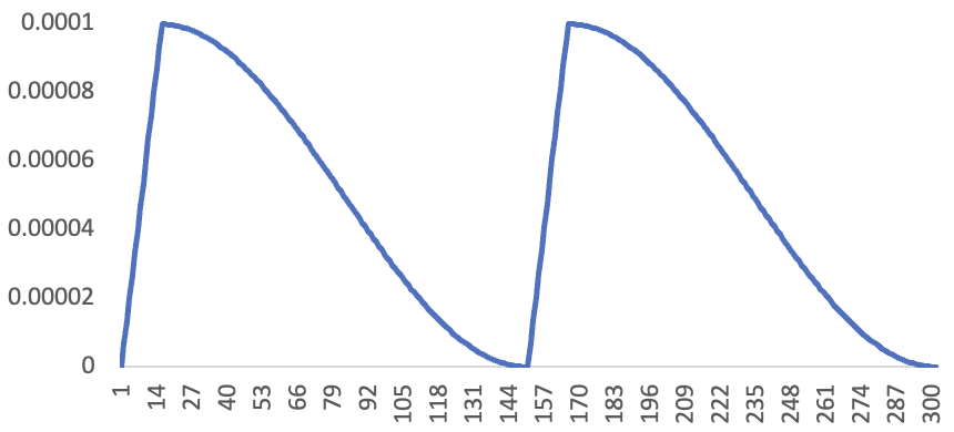
Nowadays this kind of schedule is not that common, but it’s an approach that saw a lot of success after it was created by Leslie Smith, who discussed it in his 2015 paper Cyclical Learning Rates for Training Neural Networks.
And here’s the crazy-looking training and validation loss curves we saw as a result:
The only thing that we have come up with (so far!) that fully explains this picture is that the hypothesis is correct: the model is rapidly learning to recognise examples even just seeing them once. Let’s work through each part of the loss curve in turn…
Looking at the first epoch, this looks like a very standard loss curve. We have the learning rate warming up over the first 10% of the epoch, and then gradually decreasing following a cosine schedule. Once the LR comes up to temperature, the training and validation loss rapidly decrease, and then they both slow down as the LR decreases and the “quick wins” are captured.
The second epoch is where it gets interested. We’re not re-shuffling the dataset at the start of the epoch, so those first batches of the second epoch are when the learning rate was still warming up. That’s why we don’t see an immediate step-change like we did from epoch 2 to 3 in the very first loss curve we showed – these batches were only seen when the LR was low, so it couldn’t learn much.
Towards the end of that first 10% of the epoch, the training loss plummets, because the LR was high when these batches were seen during the first epoch, and the model has learned what they look like. The model quickly learns that it can very confidentally guess the correct answer.
But during this time, validation loss suffers. That’s because although the model is getting very confident, it’s not actually getting any better at making predictions. It has simply memorised the dataset, but isn’t improving at generalizing. Over-confident predictions cause validation loss to get worse, because the loss function penalizes more confident errors higher.
The end of the curve is where things get particularly interesting. The training loss starts getting worse – and that really never ought to happen! In fact, neither of us remember ever seeing such a thing before when using a reasonable LR.
But actually, this makes perfect sense under the memorization hypothesis: these are the batches that the model saw at a time when the LR had come back down again, so it wasn’t able to memorize them as effectively. But the model is still over-confident, because it has just got a whole bunch of batches nearly perfectly correct, and hasn’t yet adjusted to the fact that it’s now seeing batches that it didn’t have a chance to learn so well.
It gradually recalibrates to a more reasonable level of confidence, but it takes a while, because the LR is getting lower and lower. As it recalibrates, the validation loss comes back down again.
For our next experiment, we tried 1cycle training over 3 epochs, instead of CLR – that is, we did a single LR warmup for 10% of batches at the start of training, and then decayed the LR over the remaining batches following a cosine schedule. Previously, we did a separate warmup and decay cycle for each epoch. Also, we increased the LoRA rank, resulting in slower learning. Here’s the resulting loss curve:
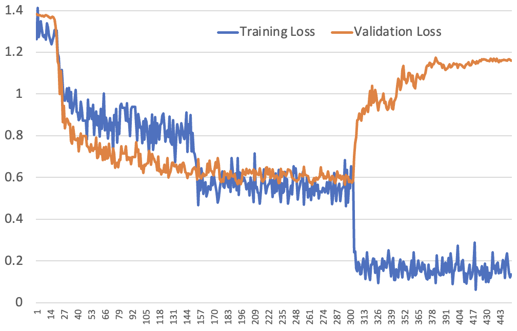
The shape largely follows what we’d expect, based on the previous discussion, except for one thing: the validation loss does not jump up at epoch 2 – it’s not until epoch 3 that we see that jump. However previously the training loss was around 0.2 by the 2nd epoch, which is only possible when it’s making highly confident predictions. In the 1cycle example it doesn’t make such confident predictions until the third epoch, and we don’t see the jump in validation loss until that happens.
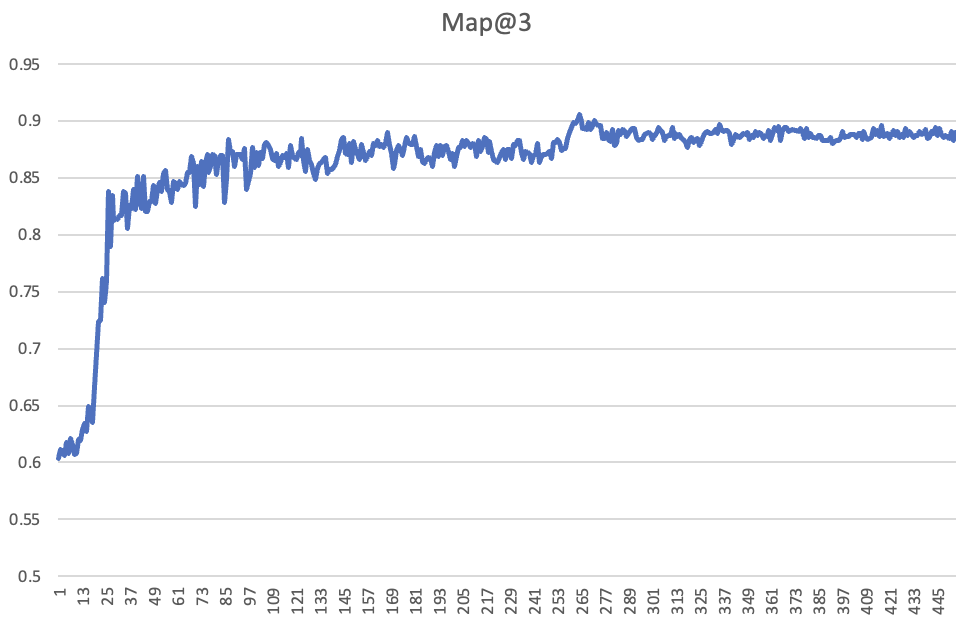
It’s important to note that the validation loss getting worse doesn’t mean that we’re over-fitting in practice. What we generally care about is accuracy, and it’s fine if the model is over-confident. In the Kaggle competition the metric used for the leaderboard is Mean Average Precision @ 3 (MAP@3), which is the accuracy of the ranked top-3 multiple-choice predictions made my the model. Here’s the validation accuracy per batch of the 1cycle training run shown in the previous chart – as you see, it keeps improving, even although the validation loss got worse in the last epoch:
If you’re interested in diving deeper, take a look at this report where Johno shares logs from some additional examples, along with a notebook for those who’d like to see this effect in action for themselves.
How could the memorization hypothesis be true?
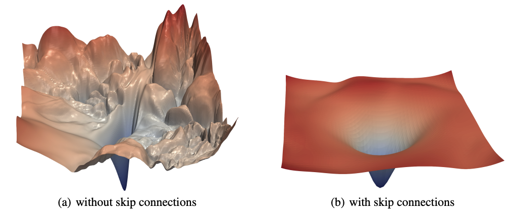
There is no fundamental law that says that neural networks can’t learn to recognise inputs from a single example. It’s just what researchers and practitioners have generally found to be the case in practice. It takes a lot of examples because the loss surfaces that we’re trying to navigate using stochastic gradient descent (SGD) are too bumpy to be able to jump far at once. We do know, however, that some things can make loss surfaces smoother, such as using residual connections, as shown in the classic Visualizing the Loss Landscape of Neural Nets paper (Li et al, 2018).
It could well be the case that pre-trained large language models have extremely smooth loss surfaces in areas close to the minimal loss, and that a lot of the fine-tuning work done in the open source community is in this area. This is based on the underlying premise surrounding the original development of fine-tuned universal language models. These models were first documented in the ULMFiT paper back in 2018 by one of us (Jeremy) and Sebastian Ruder. The reason Jeremy originally built the ULMFiT algorithm is because it seemed necessary that any model that could do a good job of language modeling (that is, predicting the next word of a sentence) would have to build a rich hierarchy of abstractions and capabilities internally. Furthermore, Jeremy believed that this hierarchy could then be easily adapted to solve other tasks requiring similar capabilities using a small amount of fine-tuning. The ULMFiT paper demonstrated for the first time that this is indeed exactly what happens.
Large language models, which today are orders of magnitude bigger than those studied in ULMFiT, must have an even richer hierarchy of abstractions. So fine-tuning one of these models to, for instance, answer multiple-choice questions about science, can largely harness capabilities and knowledge that is already available in the model. It’s just a case of surfacing the right pieces in the right way. These should not require many weights to be adjusted very much.
Based on this, it’s perhaps not surprising to think that a pre-trained language model with a small random classification head could be in a part of the weight space where the loss surface smoothly and clearly points exactly in the direction of a good weight configuration. And when using the Adam optimiser (as we did), having a consistent and smooth gradient results in effective dynamic learning rate going up and up, such that steps can get very big.
What now?
Having a model that learns really fast sounds great – but actually it means that a lot of basic ideas around how to train models may be turned on their head! When models train very slowly, we can train them for a long time, using a wide variety of data, for multiple epochs, and we can expect that our model will gradually pull out generalisable information from the data we give it.
But when models learn this fast, the catastrophic forgetting problem may suddenly become far more pronounced. For instance, if a model sees ten examples of a very common relationship, and then one example of a less common counter-example, it may well remember the counter-example instead of just slightly downweighting its memory of the original ten examples.
It may also be the case now that data augmentation is now less useful for avoiding over-fitting. Since LLMs are so effective at pulling out representations of the information they’re given, mixing things up by paraphrasing and back-translation may now not make much of a difference. The model would be effectively getting the same information either way.
Perhaps we can mitigate these challenges by greatly increasing our use of techniques such as dropout (which is already used a little in fine-tuning techniques such as LoRA) or stochastic depth (which does not seem to have been used in NLP to any significant extent yet).
Alternatively, maybe we just need to be careful to use rich mixtures of datasets throughout training, so that our models never have a chance to forget. Although Llama Code, for instance, did suffer from catastrophic forgetting (as it got better at code, it got much worse at everything else), it was fine-tuned with only 10% of non-code data. Perhaps with something closer to a 50/50 mix it would have been possible to get just as good at coding, without losing its existing capabilities.
If you come up with any alternative hypotheses, and are able to test them, or if you find any empirical evidence that the memorization hypothesis is wrong, please do let us know! We’re also keen to hear about other work in this space (and apologies if we failed to reference any prior work here), and any ideas about how (if at all) we should adjust how we train and use these models based on these observations. We’ll be keeping an eye on replies to this twitter thread, so please respond there if you have any thoughts or questions.